
Top Rated items in this list as voted by talkKs Readers
- Visualize Data with Sparkline : 1 vote
Google Sheets is a powerful spreadsheet application that is used by millions of people every day. It is perfect for both business and personal needs and is a great tool to store or organize data, make calculations, and collaborate with others. It’s a web based application, so unlike Microsoft Excel desktop software, Google Sheets allows to work on spreadsheet tasks across multiple locations and devices. You just need to have an internet connection to start or resume the work.
Google Sheets comes with many features that are popular among typical spreadsheet softwares like MS Excel,. This includes functions that allow you to filter data through queries, add conditional formatting, create charts and graphs from the data in your sheet, format data as pivot tables and summaries, use formulas for math calculations, and add comments on cells to share ideas with others working on the same sheet at the same time. Many people know only the most basic functions in Google Sheets. In this article, we are going to teach you some Google Sheets tips and tricks that will come in handy for your work.
So without further ado, here are our top picks for Google Sheets tips that not only saves your time, your sanity too!
Use Up/Down vote buttons and comment section under each list item to tell us your opinion and rank these based on your preference.
-
1 Wrap Text in Certain Cells
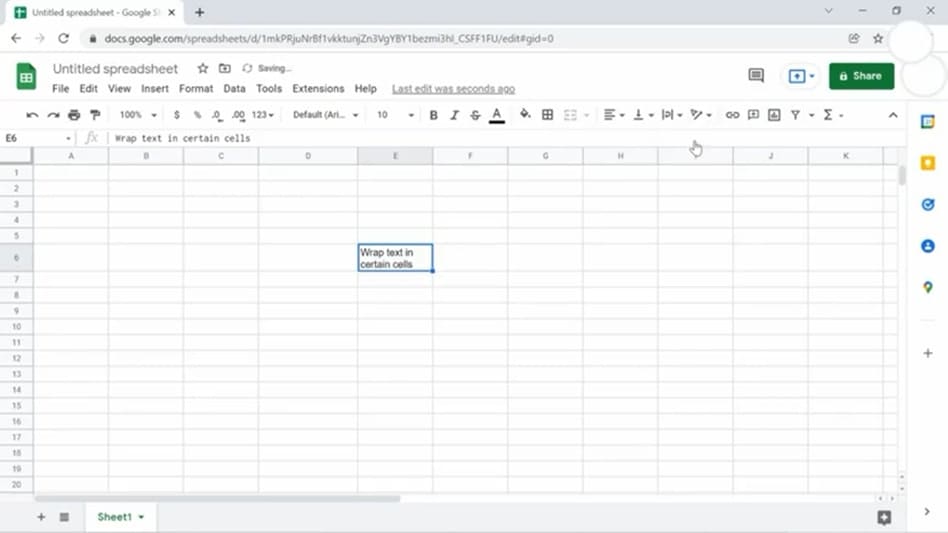
If a cell has a long sentence or string, it tends to overflow to the adjacent cells. You can avoid this by using the wrap function in Google Sheets. To do this, first, select the cell you want to wrap, then go to Format → Text Wrapping →Wrap. Another method to wrap text is to click on the 'Wrap Text' option in the toolbar.
Leave a Reply -
2 Capitalize Names in Google Sheets
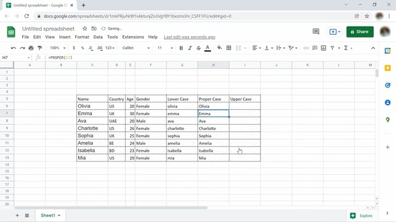
We all know that proper names start with capital letters, but it's natural to forget capitalizing when typing a lot of names. But don't worry! Google Sheets has an in-built function called PROPER that helps you with capitalizing names. To use this function, you can use the formula =UPPER("cell reference"). This will automatically add proper capitalization to your selected cells.
-
3 Quickly Change the Number format in Google Sheets
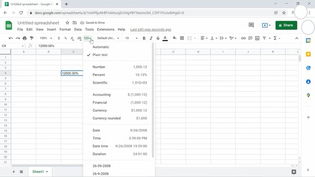
You can easily change the format of a number using the main toolbar. For example, if you have just typed in some numbers in a column and want to change it to a percentage, you don't have to manually type the % mark. You can just select the percentage icon in the main toolbar. There are many different number formats in the main toolbar, including percentages, decimals, and currencies.
-
4 Add Checkboxes to Google Sheets
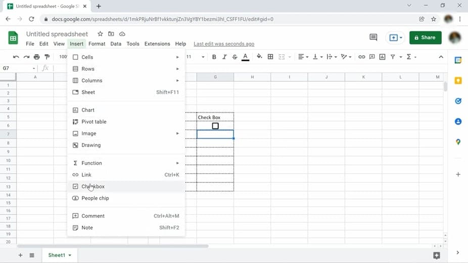
Sometimes, you might want to add checkboxes, which usually help you to add yes or no (or true or false) answers. To add these, first select the cell, then go to Format, and select Checkbox. Checkboxes can make your sheet more fun and interactive.
-
5 Add a Drop-down Box to Limit Choices
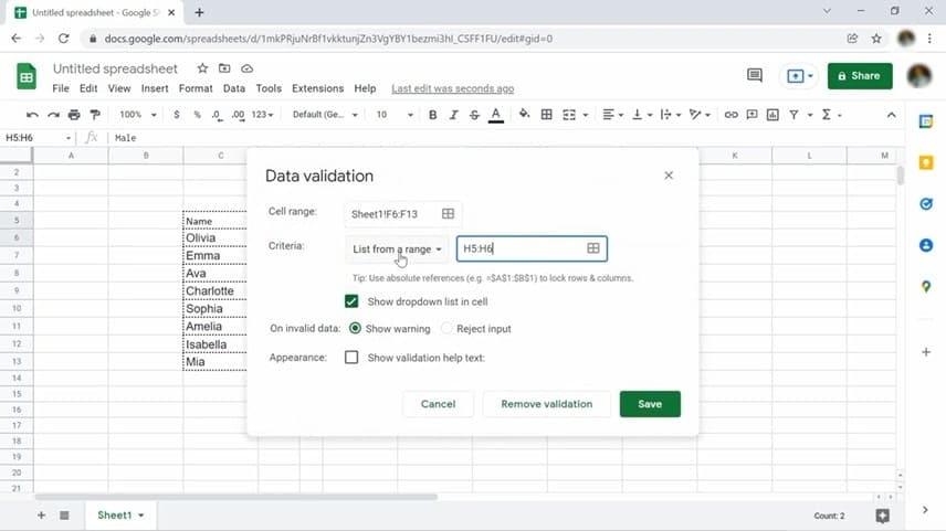
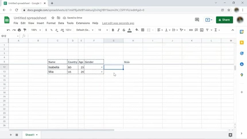
If the entry in a certain column has a limited number of choices, you can easily limit the possible choices and save time by creating a drop-down in Google sheets. First, select the cells where you want to create the drop-down box. Next, click on Data → Data Validation. Then you will have to fill in the information.
In the 'Criteria' section, you can choose an option that suits you. If you choose 'List from a range,' you have to choose the cells that list the choices to be included in the drop-down box. You can also choose 'List of items' and enter the choices, separated by commas (no spaces).
-
6 Lock Header Rows
When you are looking at a long spreadsheet, you might sometimes forget what the individual columns are for. But you can easily freeze or lock the header row with a few clicks of the mouse. Take your cursor to the top-left corner of the worksheet, where there is a blank grey box with two thick grey lines. When you hover over the horizontal grey line, your cursor will change to a hand icon. Now hold the left mouse key and drag this grey line down. Since you only want to lock the header row (top of the row), you have to drag this line just below the first row. If you want to freeze the first few rows, you can also drag the line to the end of the first few lines.
There is another method to freeze cells in a Google spreadsheet. Click on 'View' on the menu and choose 'Freeze.' Then you can select '1 row'. -
7 Copy and Paste Values, Instead of Formulas
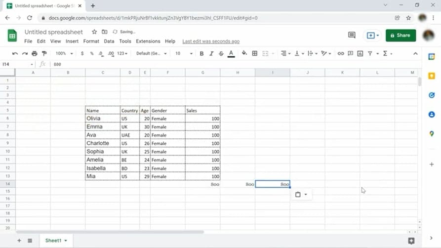
When you copy and paste a value you obtained using a formula to another Google sheet or a cell that is far away from the original cell, the value can change. This is because what you are copying is the formula, not the value itself. You can easily copy and paste a value by using the keyboard shortcut: CTRL+C / CTRL+ Shift +V. Another way to copy and paste values is right clicking on the cells where you have to paste the value and select 'Paste Special' from the menu that appears. This will open a sub-menu with different paste options. Select 'Paste values only' from these options. Now your value will automatically be pasted.
-
8 Copy the Format of One Cell to Another Cell
In Google sheets, you can easily copy the format of one cell on another cell without changing the data in both cells. To do this with keyboard shortcuts, first select the cells you want to copy, press Ctrl + C, click on the destination cells, and click Ctrl + Alt + V.
-
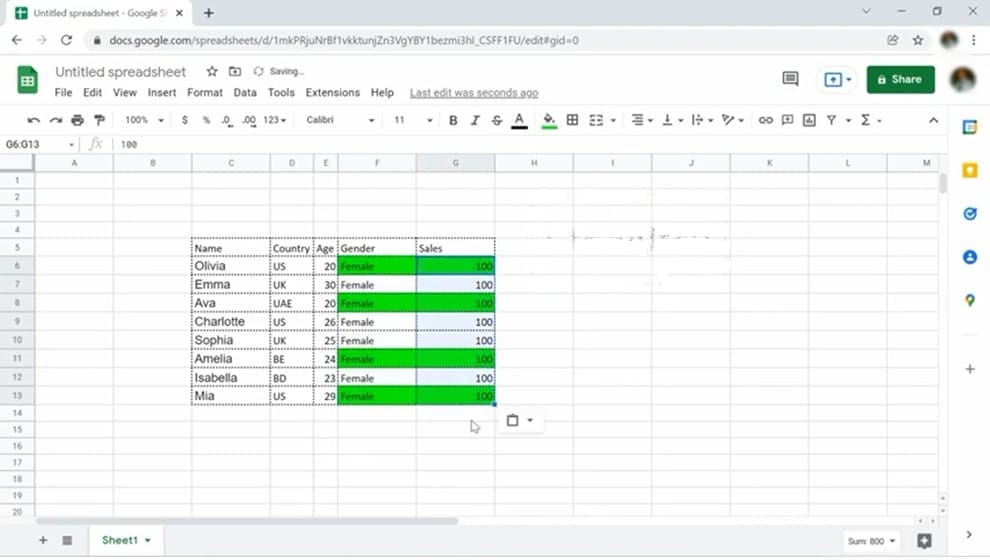
9 Use Conditional Formatting in Google Sheets
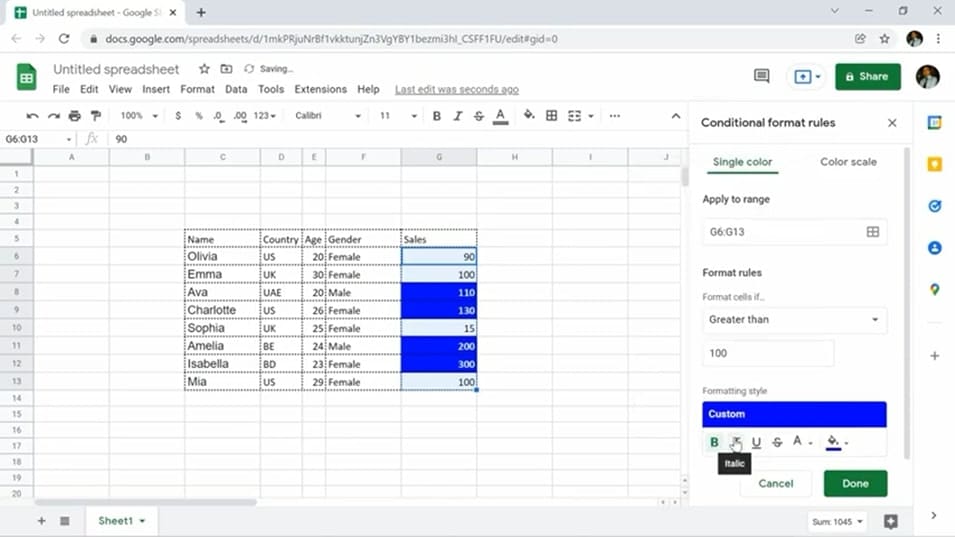
Google Sheets gives you the function of Conditional formatting, which allows formatting a cell in a certain way when certain conditions are met. This formatting usually involves visual changes – highlighting, bolding, italicizing, etc. To set up conditional formatting, select the cells you want to format, then select 'Format' in the navigation menu, and click on 'Conditional Formatting.' Then set your Format rules and Format style.
-
10 Copy and Paste an Array with Rows and Columns Flipped
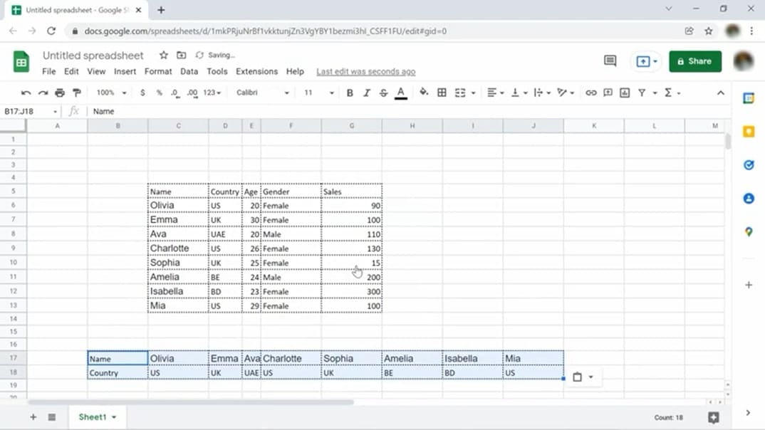
If you want to copy an array to another location in Google Sheets but want it with rows and columns flipped, you can easily copy the cells you want and then right click on the first cell where you want to paste the array. Then you will get the right-click menu. From here, select Paste Special → Transposed. Your array will be automatically pasted with rows and columns flipped.
-
11 Access a List of Keyboard Shortcuts in Google Sheets
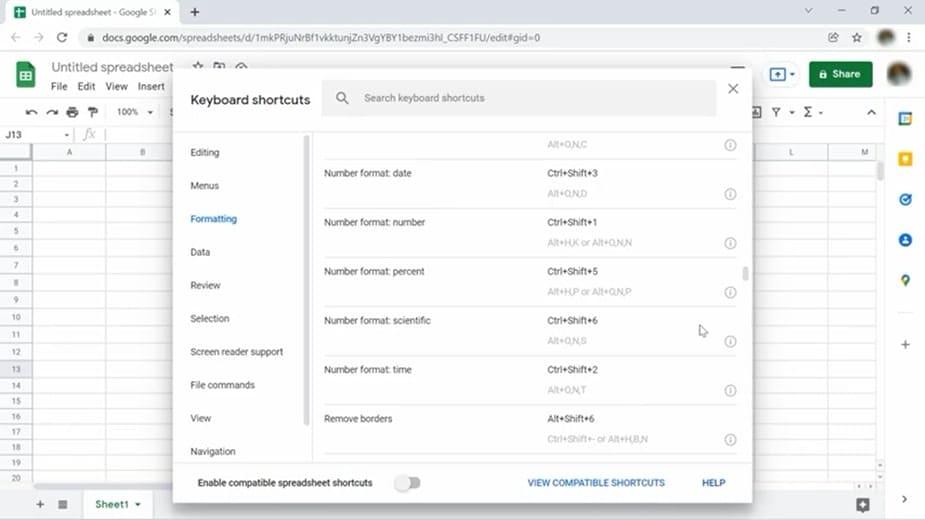
Google Sheets have many keyboard shortcuts. But it's not easy to remember them all. You can simply access the list of shortcuts in Google sheets by pressing Ctrl + /. This shortcut will open the window below, which shows all shortcuts grouped by category.
-
12 Translate Words Using Google Translate
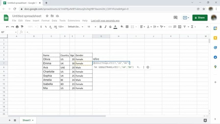
Did you know that Google Sheets has a built-in google translate function that you could use to translate simple words? All you have to do is select the cell you want to translate, then use the following formula in another cell to translate it.
=GOOGLETRANSLATE(cell with text, "source language", "target language")
Here, the source language is the language your text is currently in, and the target language is the language you want to translate to. -
13 Verify a Valid Email Address
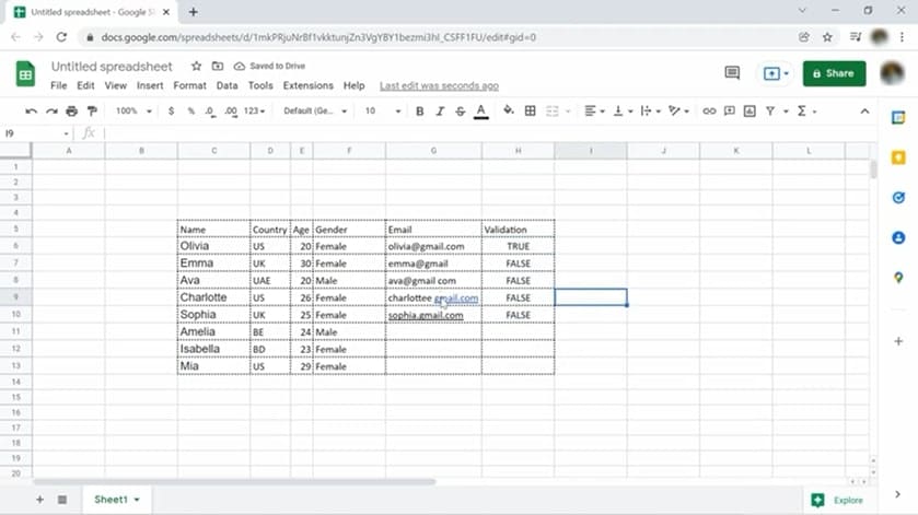
If you are typing email addresses in Google Sheets, you have to make sure that the data you entered is correct. The easiest way to do this is by confirming that the email address format is correct. You can do this by Data Verification. First, select the cells where you want to apply data validation. Then, select Data → Data Validation from the navigation menu. Then you will see a small window you have to fill in. Make sure the Cell range is correct and choose 'Text' and 'contains' for 'Criteria.' Next, enter the @ symbol in the box next to 'contains.' Next, for 'On Invalid Data' you can either choose 'Show Warning' or 'Reject Input.'
-
14 Easily Insert Links to External Websites
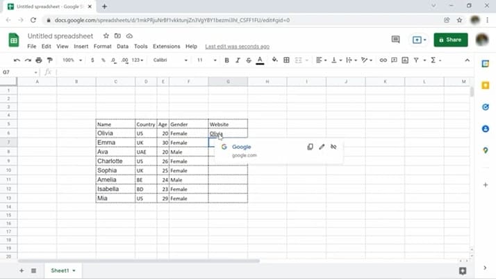
Google Sheets has a built-in hyperlink function to link to external sites. To add a hyperlink, select the cell where you want to insert the link and type the following formula:
=HYPERLINK(URL, LINK_LABEL)
Here, URL is the link to the external site, and the link label is the text you want to display on the cell. -
15 Ensure that Spelling is Correct in Google Sheets
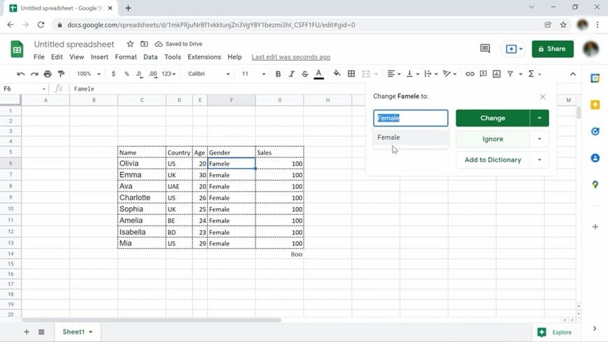
You can easily correct all your spelling mistakes in Google Sheets by using the spelling function. First, select the cell range you want to check. Then click on the Tools tab and select Spelling. Then Google will automatically detect your errors and suggest the corrections.
-
16 Visualize Data with Sparkline
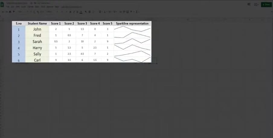
In Google Sheets, you can easily visualize your data in the form of tiny line graphs that illustrates a trend. We call this a Sparkline. All you have to do to add a Sparkline to your data is click on the cell you want to insert it and type =SPARKLINE, and enter the range of values enclosed in brackets. When you ENTER, you will get a small line graph visualizing your data.
-
17 Send Emails with a Comment
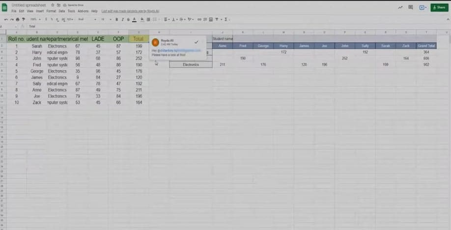
When you add a comment to a Google Sheet, you can also send someone an email notification of the comment. To do this, first right-click on the cell you want to comment and select 'Comment.' Type your comment in the small pop-up window that appears, and type @email address. By doing this, the person you mentioned will receive an email notification.
-
18 Integrate Google Forms with Google Sheets
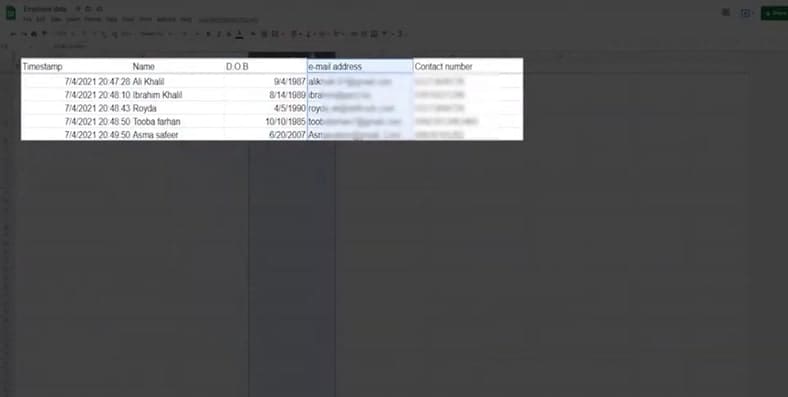
If you want to create a table in Google Sheets with the data taken from Google Forms, you don't have to do this manually. You can directly send data from Google Forms into Google Sheets by clicking the sheet icon on the top right of the form. Then enter the name of the form, and a Google Sheet tab automatically opens with all the data of the form. The sheet will also have the timestamp, which shows the time when the data was entered.
-
19 Import Web Data Using IMPORTHTML
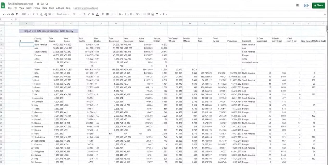
Not many people know that Google Sheets offers a special function to import data from a table or list on an HTML page or site. This function is known as IMPORTHTML. It automatically pulls data from a website into Google Sheets.
First, copy the URL of the website you want to extract data from. Next, go to Insert tab → Function→ Web →IMPORTHTML. This will open a pop-up window. Next to IMPORTHTML, you will see brackets. Put inverted commas inside the brackets and paste the URL you copied earlier between them. Type another set of inverted commas and specify the query. Hit ENTER, and the entire table from the website will be imported to the sheet within seconds. -
20 Display Formulas as Text Strings
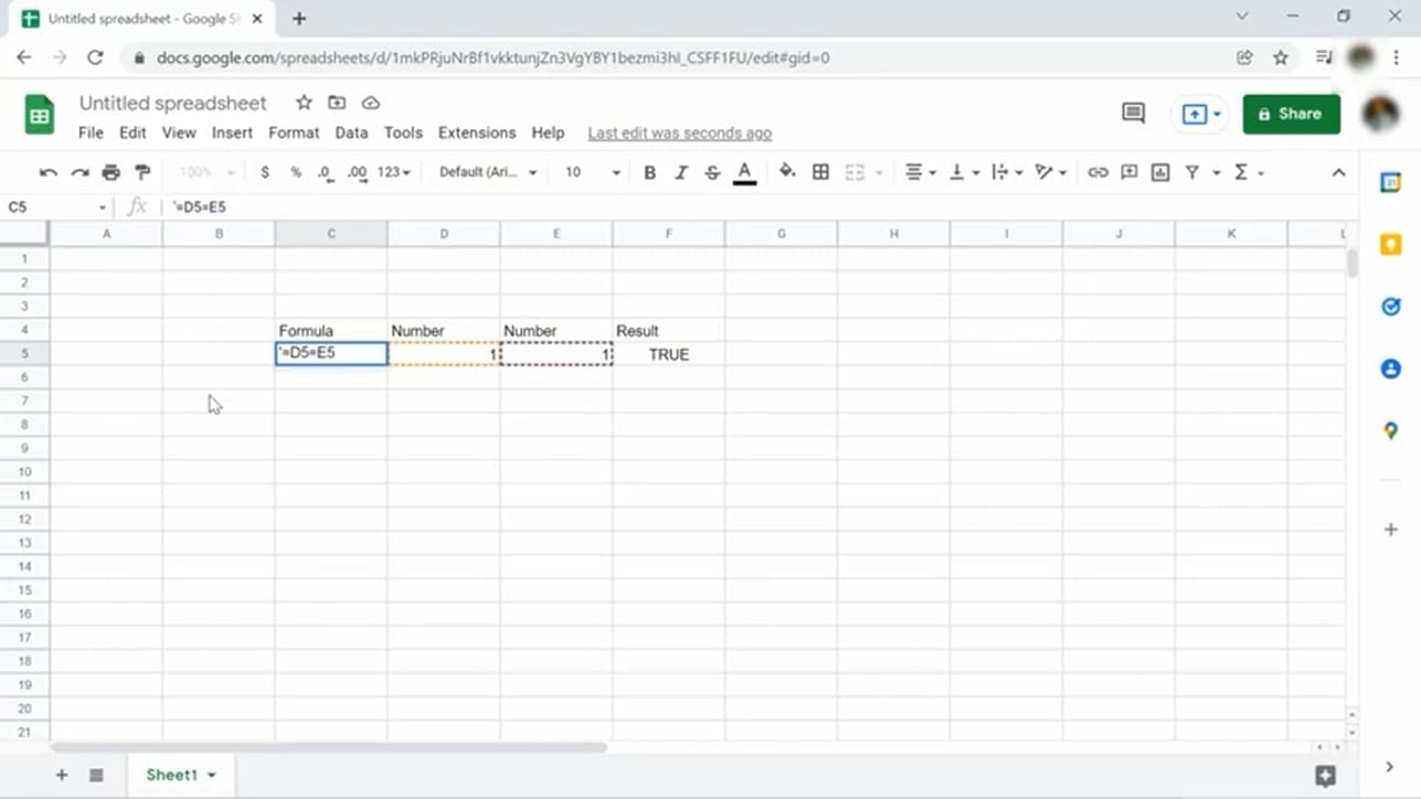
Sometimes, you might want to display a formula on a cell to explain the calculations you have made on another cell. But once you enter this formula on a cell, Google Sheets will automatically run it as an actual formula.
To avoid this processing, you can insert an apostrophe before typing the formula. This will display your formula as a text string.